Elliptic functions

Elliptic functions historically comprise the elliptic integrals and their inverses, and originate from the problem of computing the arc length of an ellipse. From a more modern point of view, an elliptic function is defined as a doubly periodic function, i.e. a function which satisfies

\[f(z + 2 \omega_1) = f(z + 2 \omega_2) = f(z)\]

for some half-periods \(\omega_1, \omega_2\) with \(\mathrm{Im}[\omega_2 / \omega_1] > 0\). The classical examples include the Jacobi elliptic functions and the Weierstrass elliptic functions. More broadly, this section includes quasi-doubly periodic functions (such as the Jacobi theta functions) and other functions useful in the study of elliptic functions.

Many different conventions for the arguments of elliptic functions are in use. It is even standard to use different parameterizations for different functions in the same text or software (and mpmath is no exception). The usual parameters are the elliptic nome \(q\), which usually must satisfy \(|q| < 1\); the elliptic parameter \(m\) (an arbitrary complex number); the elliptic modulus \(k\) (an arbitrary complex number); and the half-period ratio \(\tau\), which usually must satisfy \(\mathrm{Im}[\tau] > 0\). Elliptic functions may also be parameterized by half-periods \(\omega_1, \omega_2\), where \(\tau = \omega_2 / \omega_1\), or by Weierstrass invariants \(g_2, g_3\). These quantities can be expressed in terms of each other using the following relations:

\[m = k^2\]

\[\tau = i \frac{K(1-m)}{K(m)}\]

\[q = e^{i \pi \tau}\]

\[k = \frac{\vartheta_2^2(q)}{\vartheta_3^2(q)}\]

In addition, an alternative definition is used for the nome in number theory, which we here denote by q-bar:

\[\bar{q} = q^2 = e^{2 i \pi \tau}\]

For convenience, mpmath provides functions to convert between the various parameters, including half-periods and Weierstrass invariants where applicable (qfrom(), mfrom(), kfrom(), taufrom(), qbarfrom()).

References

1. [AbramowitzStegun]

2. [WhittakerWatson]

Elliptic arguments

mpmath.qfrom(q=None, m=None, k=None, tau=None, qbar=None, g2=None, g3=None, omega1=None, omega2=None)

Returns the elliptic nome \(q\), given any of \(q, m, k, \tau, \bar{q}\). It may also be computed from both Weierstrass invariants \(g_2, g_3\), or both half-periods \(\omega_1, \omega_2\):

>>> from mpmath import mp, qfrom, mfrom, kfrom, taufrom, qbarfrom
>>> mp.dps = 25
>>> mp.pretty = True
>>> qfrom(q=0.25)
0.25
>>> qfrom(m=mfrom(q=0.25))
0.25
>>> qfrom(k=kfrom(q=0.25))
0.25
>>> qfrom(tau=taufrom(q=0.25))
(0.25 + 0.0j)
>>> qfrom(qbar=qbarfrom(q=0.25))
0.25
>>> qfrom(omega1=1, omega2=0.5j)
(0.2078795763507619085469556 + 0.0j)

mpmath.qbarfrom(q=None, m=None, k=None, tau=None, qbar=None, g2=None, g3=None, omega1=None, omega2=None)

Returns the number-theoretic nome \(\bar q\), given any of \(q, m, k, \tau, \bar{q}\), both Weierstrass invariants \(g_2, g_3\), or both half-periods \(\omega_1, \omega_2\):

>>> from mpmath import (mp, qbarfrom, qfrom, extraprec, mfrom,
...                     kfrom, taufrom)
>>> mp.dps = 25
>>> mp.pretty = True
>>> qbarfrom(qbar=0.25)
0.25
>>> qbarfrom(q=qfrom(qbar=0.25))
0.25
>>> qbarfrom(m=extraprec(20)(mfrom)(qbar=0.25))  # ill-conditioned
0.25
>>> qbarfrom(k=extraprec(20)(kfrom)(qbar=0.25))  # ill-conditioned
0.25
>>> qbarfrom(tau=taufrom(qbar=0.25))
(0.25 + 0.0j)
>>> qbarfrom(omega1=1, omega2=0.5j)
(0.04321391826377224977441774 + 0.0j)

mpmath.mfrom(q=None, m=None, k=None, tau=None, qbar=None, g2=None, g3=None, omega1=None, omega2=None)

Returns the elliptic parameter \(m\), given any of \(q, m, k, \tau, \bar{q}\), both Weierstrass invariants \(g_2, g_3\), or both half-periods \(\omega_1, \omega_2\):

>>> from mpmath import mp, mfrom, qfrom, kfrom, taufrom, qbarfrom, taylor
>>> mp.dps = 25
>>> mp.pretty = True
>>> mfrom(m=0.25)
0.25
>>> mfrom(q=qfrom(m=0.25))
0.25
>>> mfrom(k=kfrom(m=0.25))
0.25
>>> mfrom(tau=taufrom(m=0.25))
(0.25 + 0.0j)
>>> mfrom(qbar=qbarfrom(m=0.25))
0.25
>>> mfrom(omega1=1, omega2=0.5j)
(0.9705627484771405856202647 + 0.0j)

As \(q \to 1\) and \(q \to -1\), \(m\) rapidly approaches \(1\) and \(-\infty\) respectively:

>>> mfrom(q=0.75)
0.9999999999999798332943533
>>> mfrom(q=-0.75)
-49586681013729.32611558353
>>> mfrom(q=1)
1.0
>>> mfrom(q=-1)
-inf

The inverse nome as a function of \(q\) has an integer Taylor series expansion:

>>> taylor(lambda q: mfrom(q), 0, 7)
[0.0, 16.0, -128.0, 704.0, -3072.0, 11488.0, -38400.0, 117632.0]

mpmath.kfrom(q=None, m=None, k=None, tau=None, qbar=None, g2=None, g3=None, omega1=None, omega2=None)

Returns the elliptic modulus \(k\), given any of \(q, m, k, \tau, \bar{q}\), both Weierstrass invariants \(g_2, g_3\), or both half-periods \(\omega_1, \omega_2\):

>>> from mpmath import mp, kfrom, mfrom, qfrom, taufrom, qbarfrom
>>> mp.dps = 25
>>> mp.pretty = True
>>> kfrom(k=0.25)
0.25
>>> kfrom(m=mfrom(k=0.25))
0.25
>>> kfrom(q=qfrom(k=0.25))
0.25
>>> kfrom(tau=taufrom(k=0.25))
(0.25 + 0.0j)
>>> kfrom(qbar=qbarfrom(k=0.25))
0.25
>>> kfrom(omega1=1, omega2=0.5j)
(0.985171431009416038689502 + 0.0j)

As \(q \to 1\) and \(q \to -1\), \(k\) rapidly approaches \(1\) and \(i \infty\) respectively:

>>> kfrom(q=0.75)
0.9999999999999899166471767
>>> kfrom(q=-0.75)
(0.0 + 7041781.096692038332790615j)
>>> kfrom(q=1)
1
>>> kfrom(q=-1)
(0.0 + infj)

mpmath.taufrom(q=None, m=None, k=None, tau=None, qbar=None, g2=None, g3=None, omega1=None, omega2=None)

Returns the elliptic half-period ratio \(\tau\), given any of \(q, m, k, \tau, \bar{q}\), both Weierstrass invariants \(g_2, g_3\), or both half-periods \(\omega_1, \omega_2\):

>>> from mpmath import mp, taufrom, qfrom, mfrom, kfrom, qbarfrom
>>> mp.dps = 25
>>> mp.pretty = True
>>> taufrom(tau=0.5j)
(0.0 + 0.5j)
>>> taufrom(q=qfrom(tau=0.5j))
(0.0 + 0.5j)
>>> taufrom(m=mfrom(tau=0.5j))
(0.0 + 0.5j)
>>> taufrom(k=kfrom(tau=0.5j))
(0.0 + 0.5j)
>>> taufrom(qbar=qbarfrom(tau=0.5j))
(0.0 + 0.5j)
>>> taufrom(omega1=1, omega2=0.5j)
(0.0 + 0.5j)

Legendre elliptic integrals

mpmath.ellipk(x, *, prec=None, dps=None, rounding=None)

Evaluates the complete elliptic integral of the first kind, \(K(m)\), defined by

\[K(m) = \int_0^{\pi/2} \frac{dt}{\sqrt{1-m \sin^2 t}} \, = \, \frac{\pi}{2} \,_2F_1\left(\frac{1}{2}, \frac{1}{2}, 1, m\right).\]

Note that the argument is the parameter \(m = k^2\), not the modulus \(k\) which is sometimes used.

Plots

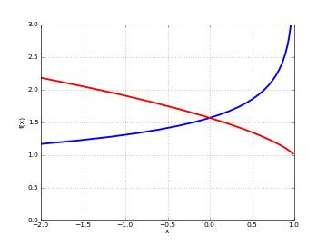
# Complete elliptic integrals K(m) and E(m)
plot([ellipk, ellipe], [-2,1], [0,3], points=600)

Examples

Values and limits include:

>>> from mpmath import mp, ellipk, inf, sin, quad, pi, hyp2f1, quad
>>> mp.dps = 25
>>> mp.pretty = True
>>> ellipk(0)
1.570796326794896619231322
>>> ellipk(inf)
(0.0 + 0.0j)
>>> ellipk(-inf)
0.0
>>> ellipk(1)
inf
>>> ellipk(-1)
1.31102877714605990523242
>>> ellipk(2)
(1.31102877714605990523242 - 1.31102877714605990523242j)

Verifying the defining integral and hypergeometric representation:

>>> ellipk(0.5)
1.85407467730137191843385
>>> quad(lambda t: (1-0.5*sin(t)**2)**-0.5, [0, pi/2])
1.85407467730137191843385
>>> pi/2*hyp2f1(0.5,0.5,1,0.5)
1.85407467730137191843385

Evaluation is supported for arbitrary complex \(m\):

>>> ellipk(3+4j)
(0.9111955638049650086562171 + 0.6313342832413452438845091j)

A definite integral:

>>> quad(ellipk, [0, 1])
2.0

mpmath.ellipf(phi, m)

Evaluates the Legendre incomplete elliptic integral of the first kind

\[F(\phi,m) = \int_0^{\phi} \frac{dt}{\sqrt{1-m \sin^2 t}}\]

or equivalently

\[F(\phi,m) = \int_0^{\sin \phi} \frac{dt}{\left(\sqrt{1-t^2}\right)\left(\sqrt{1-mt^2}\right)}.\]

The function reduces to a complete elliptic integral of the first kind (see ellipk()) when \(\phi = \frac{\pi}{2}\); that is,

\[F\left(\frac{\pi}{2}, m\right) = K(m).\]

In the defining integral, it is assumed that the principal branch of the square root is taken and that the path of integration avoids crossing any branch cuts. Outside \(-\pi/2 \le \Re(\phi) \le \pi/2\), the function extends quasi-periodically as

\[F(\phi + n \pi, m) = 2 n K(m) + F(\phi,m), n \in \mathbb{Z}.\]

Plots

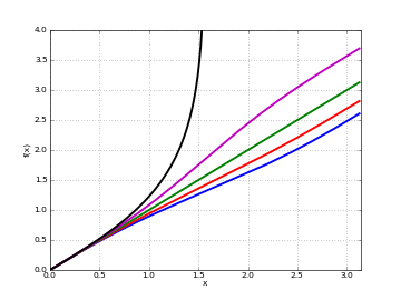
# Elliptic integral F(z,m) for some different m
f1 = lambda z: ellipf(z,-1)
f2 = lambda z: ellipf(z,-0.5)
f3 = lambda z: ellipf(z,0)
f4 = lambda z: ellipf(z,0.5)
f5 = lambda z: ellipf(z,1)
plot([f1,f2,f3,f4,f5], [0,pi], [0,4])

Examples

Basic values and limits:

>>> from mpmath import (mp, ellipf, log, sec, tan, pi, eps, ellipk,
...                     sin, appellf1, quad)
>>> mp.dps = 25
>>> mp.pretty = True
>>> ellipf(0,1)
0.0
>>> ellipf(0,0)
0.0
>>> ellipf(1,0)
1.0
>>> ellipf(2+3j,0)
(2.0 + 3.0j)
>>> ellipf(1,1)
1.226191170883517070813061
>>> log(sec(1)+tan(1))
1.226191170883517070813061
>>> ellipf(pi/2, -0.5)
1.415737208425956198892166
>>> ellipk(-0.5)
1.415737208425956198892166
>>> ellipf(pi/2+eps, 1)
inf
>>> ellipf(-pi/2-eps, 1)
inf
>>> ellipf(1.5, 1)
3.340677542798311003320813

Comparing with numerical integration:

>>> z,m = 0.5, 1.25
>>> ellipf(z,m)
0.5287219202206327872978255
>>> quad(lambda t: (1-m*sin(t)**2)**(-0.5), [0,z])
0.5287219202206327872978255

The arguments may be complex numbers:

>>> ellipf(3j, 0.5)
(0.0 + 1.713602407841590234804143j)
>>> ellipf(3+4j, 5-6j)
(1.269131241950351323305741 - 0.3561052815014558335412538j)
>>> z,m = 2+3j, 1.25
>>> k = 1011
>>> ellipf(z+pi*k,m)
(4086.184383622179764082821 - 3003.003538923749396546871j)
>>> ellipf(z,m) + 2*k*ellipk(m)
(4086.184383622179764082821 - 3003.003538923749396546871j)

For \(|\Re(z)| < \pi/2\), the function can be expressed as a hypergeometric series of two variables (see appellf1()):

>>> z,m = 0.5, 0.25
>>> ellipf(z,m)
0.5050887275786480788831083
>>> sin(z)*appellf1(0.5,0.5,0.5,1.5,sin(z)**2,m*sin(z)**2)
0.5050887275786480788831083

mpmath.ellipe(*args)

Called with a single argument \(m\), evaluates the Legendre complete elliptic integral of the second kind, \(E(m)\), defined by

\[E(m) = \int_0^{\pi/2} \sqrt{1-m \sin^2 t} \, dt \,=\, \frac{\pi}{2} \,_2F_1\left(\frac{1}{2}, -\frac{1}{2}, 1, m\right).\]

Called with two arguments \(\phi, m\), evaluates the incomplete elliptic integral of the second kind

\[E(\phi,m) = \int_0^{\phi} \sqrt{1-m \sin^2 t} \, dt = \int_0^{\sin z} \frac{\sqrt{1-mt^2}}{\sqrt{1-t^2}} \, dt.\]

The incomplete integral reduces to a complete integral when \(\phi = \frac{\pi}{2}\); that is,

\[E\left(\frac{\pi}{2}, m\right) = E(m).\]

In the defining integral, it is assumed that the principal branch of the square root is taken and that the path of integration avoids crossing any branch cuts. Outside \(-\pi/2 \le \Re(z) \le \pi/2\), the function extends quasi-periodically as

\[E(\phi + n \pi, m) = 2 n E(m) + E(\phi,m), n \in \mathbb{Z}.\]

Plots

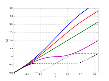
# Elliptic integral E(z,m) for some different m
f1 = lambda z: ellipe(z,-2)
f2 = lambda z: ellipe(z,-1)
f3 = lambda z: ellipe(z,0)
f4 = lambda z: ellipe(z,1)
f5 = lambda z: ellipe(z,2)
plot([f1,f2,f3,f4,f5], [0,pi], [0,4])

Examples for the complete integral

Basic values and limits:

>>> from mpmath import (mp, ellipe, inf, quad, sqrt, sin, pi,
...                     hyp2f1, appellf1)
>>> mp.dps = 25
>>> mp.pretty = True
>>> ellipe(0)
1.570796326794896619231322
>>> ellipe(1)
1.0
>>> ellipe(-1)
1.910098894513856008952381
>>> ellipe(2)
(0.5990701173677961037199612 + 0.5990701173677961037199612j)
>>> ellipe(inf)
(0.0 + infj)
>>> ellipe(-inf)
inf

Verifying the defining integral and hypergeometric representation:

>>> ellipe(0.5)
1.350643881047675502520175
>>> quad(lambda t: sqrt(1-0.5*sin(t)**2), [0, pi/2])
1.350643881047675502520175
>>> pi/2*hyp2f1(0.5,-0.5,1,0.5)
1.350643881047675502520175

Evaluation is supported for arbitrary complex \(m\):

>>> ellipe(0.5+0.25j)
(1.360868682163129682716687 - 0.1238733442561786843557315j)
>>> ellipe(3+4j)
(1.499553520933346954333612 - 1.577879007912758274533309j)

A definite integral:

>>> quad(ellipe, [0,1])
1.333333333333333333333333

Examples for the incomplete integral

Basic values and limits:

>>> ellipe(0,1)
0.0
>>> ellipe(0,0)
0.0
>>> ellipe(1,0)
1.0
>>> ellipe(2+3j,0)
(2.0 + 3.0j)
>>> ellipe(1,1)
0.8414709848078965066525023
>>> sin(1)
0.8414709848078965066525023
>>> ellipe(pi/2, -0.5)
1.751771275694817862026502
>>> ellipe(-0.5)
1.751771275694817862026502
>>> ellipe(pi/2, 1)
1.0
>>> ellipe(-pi/2, 1)
-1.0
>>> ellipe(1.5, 1)
0.9974949866040544309417234

Comparing with numerical integration:

>>> z,m = 0.5, 1.25
>>> ellipe(z,m)
0.4740152182652628394264449
>>> quad(lambda t: sqrt(1-m*sin(t)**2), [0,z])
0.4740152182652628394264449

The arguments may be complex numbers:

>>> ellipe(3j, 0.5)
(0.0 + 7.551991234890371873502105j)
>>> ellipe(3+4j, 5-6j)
(24.15299022574220502424466 + 75.2503670480325997418156j)
>>> k = 35
>>> z,m = 2+3j, 1.25
>>> ellipe(z+pi*k,m)
(48.30138799412005235090766 + 17.47255216721987688224357j)
>>> ellipe(z,m) + 2*k*ellipe(m)
(48.30138799412005235090766 + 17.47255216721987688224357j)

For \(|\Re(z)| < \pi/2\), the function can be expressed as a hypergeometric series of two variables (see appellf1()):

>>> z,m = 0.5, 0.25
>>> ellipe(z,m)
0.4950017030164151928870375
>>> sin(z)*appellf1(0.5,0.5,-0.5,1.5,sin(z)**2,m*sin(z)**2)
0.4950017030164151928870376

mpmath.ellippi(*args)

Called with three arguments \(n, \phi, m\), evaluates the Legendre incomplete elliptic integral of the third kind

\[\Pi(n; \phi, m) = \int_0^{\phi} \frac{dt}{(1-n \sin^2 t) \sqrt{1-m \sin^2 t}} = \int_0^{\sin \phi} \frac{dt}{(1-nt^2) \sqrt{1-t^2} \sqrt{1-mt^2}}.\]

Called with two arguments \(n, m\), evaluates the complete elliptic integral of the third kind \(\Pi(n,m) = \Pi(n; \frac{\pi}{2},m)\).

In the defining integral, it is assumed that the principal branch of the square root is taken and that the path of integration avoids crossing any branch cuts. Outside \(-\pi/2 \le \Re(\phi) \le \pi/2\), the function extends quasi-periodically as

\[\Pi(n,\phi+k\pi,m) = 2k\Pi(n,m) + \Pi(n,\phi,m), k \in \mathbb{Z}.\]

Plots

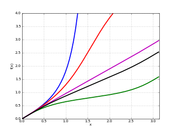
# Elliptic integral Pi(n,z,m) for some different n, m
f1 = lambda z: ellippi(0.9,z,0.9)
f2 = lambda z: ellippi(0.5,z,0.5)
f3 = lambda z: ellippi(-2,z,-0.9)
f4 = lambda z: ellippi(-0.5,z,0.5)
f5 = lambda z: ellippi(-1,z,0.5)
plot([f1,f2,f3,f4,f5], [0,pi], [0,4])

Examples for the complete integral

Some basic values and limits:

>>> from mpmath import (mp, ellippi, ellipk, inf, pi, sqrt, ellipe,
...                     log, sec, tan, ellipf)
>>> mp.dps = 25
>>> mp.pretty = True
>>> ellippi(0,-5)
0.9555039270640439337379334
>>> ellipk(-5)
0.9555039270640439337379334
>>> ellippi(inf,2)
0.0
>>> ellippi(2,inf)
0.0
>>> abs(ellippi(1,5))
inf
>>> abs(ellippi(0.25,1))
inf

Evaluation in terms of simpler functions:

>>> ellippi(0.25,0.25)
1.956616279119236207279727
>>> ellipe(0.25)/(1-0.25)
1.956616279119236207279727
>>> ellippi(3,0)
(0.0 - 1.11072073453959156175397j)
>>> pi/(2*sqrt(-2))
(0.0 - 1.11072073453959156175397j)
>>> ellippi(-3,0)
0.7853981633974483096156609
>>> pi/(2*sqrt(4))
0.7853981633974483096156609

Examples for the incomplete integral

Basic values and limits:

>>> ellippi(0.25,-0.5)
1.622944760954741603710555
>>> ellippi(0.25,pi/2,-0.5)
1.622944760954741603710555
>>> ellippi(1,0,1)
0.0
>>> ellippi(inf,0,1)
0.0
>>> ellippi(0,0.25,0.5)
0.2513040086544925794134591
>>> ellipf(0.25,0.5)
0.2513040086544925794134591
>>> ellippi(1,1,1)
2.054332933256248668692452
>>> (log(sec(1)+tan(1))+sec(1)*tan(1))/2
2.054332933256248668692452
>>> ellippi(0.25, 53*pi/2, 0.75)
135.240868757890840755058
>>> 53*ellippi(0.25,0.75)
135.240868757890840755058
>>> ellippi(0.5,pi/4,0.5)
0.9190227391656969903987269
>>> 2*ellipe(pi/4,0.5)-1/sqrt(3)
0.9190227391656969903987269

Complex arguments are supported:

>>> ellippi(0.5, 5+6j-2*pi, -7-8j)
(-0.3612856620076747660410167 + 0.5217735339984807829755815j)

Carlson symmetric elliptic integrals

mpmath.elliprf(x, y, z)

Evaluates the Carlson symmetric elliptic integral of the first kind

\[R_F(x,y,z) = \frac{1}{2} \int_0^{\infty} \frac{dt}{\sqrt{(t+x)(t+y)(t+z)}}\]

which is defined for \(x,y,z \notin (-\infty,0)\), and with at most one of \(x,y,z\) being zero.

For real \(x,y,z \ge 0\), the principal square root is taken in the integrand. For complex \(x,y,z\), the principal square root is taken as \(t \to \infty\) and as \(t \to 0\) non-principal branches are chosen as necessary so as to make the integrand continuous.

Examples

Some basic values and limits:

>>> from mpmath import (mp, elliprf, pi, inf, ellipk, ellipe,
...                     elliprd, mpf, quad, extradps, sqrt, j, gamma)
>>> mp.dps = 25
>>> mp.pretty = True
>>> elliprf(0,1,1)
1.570796326794896619231322
>>> pi/2
1.570796326794896619231322
>>> elliprf(0,1,inf)
0.0
>>> elliprf(1,1,1)
1.0
>>> elliprf(2,2,2)**2
0.5
>>> elliprf(1,0,0)
inf
>>> elliprf(0,0,1)
inf
>>> elliprf(0,1,0)
inf
>>> elliprf(0,0,0)
inf

Representing complete elliptic integrals in terms of \(R_F\):

>>> m = mpf(0.75)
>>> ellipk(m)
2.156515647499643235438675
>>> elliprf(0,1-m,1)
2.156515647499643235438675
>>> ellipe(m)
1.211056027568459524803563
>>> elliprf(0,1-m,1)-m*elliprd(0,1-m,1)/3
1.211056027568459524803563

Some symmetries and argument transformations:

>>> x,y,z = 2,3,4
>>> elliprf(x,y,z)
0.5840828416771517066928492
>>> elliprf(y,x,z)
0.5840828416771517066928492
>>> elliprf(z,y,x)
0.5840828416771517066928492
>>> k = mpf(100000)
>>> elliprf(k*x,k*y,k*z)
0.001847032121923321253219284
>>> k**(-0.5) * elliprf(x,y,z)
0.001847032121923321253219284
>>> l = sqrt(x*y) + sqrt(y*z) + sqrt(z*x)
>>> elliprf(x,y,z)
0.5840828416771517066928492
>>> 2*elliprf(x+l,y+l,z+l)
0.5840828416771517066928492
>>> elliprf((x+l)/4,(y+l)/4,(z+l)/4)
0.5840828416771517066928492

Comparing with numerical integration:

>>> x,y,z = 2,3,4
>>> elliprf(x,y,z)
0.5840828416771517066928492
>>> f = lambda t: 0.5*((t+x)*(t+y)*(t+z))**(-0.5)
>>> q = extradps(25)(quad)
>>> q(f, [0,inf])
0.5840828416771517066928492

With the following arguments, the square root in the integrand becomes discontinuous at \(t = 1/2\) if the principal branch is used. To obtain the right value, \(-\sqrt{r}\) must be taken instead of \(\sqrt{r}\) on \(t \in (0, 1/2)\):

>>> x,y,z = j-1,j,0
>>> elliprf(x,y,z)
(0.7961258658423391329305694 - 1.213856669836495986430094j)
>>> -q(f, [0,0.5]) + q(f, [0.5,inf])
(0.7961258658423391329305694 - 1.213856669836495986430094j)

The so-called first lemniscate constant, a transcendental number:

>>> elliprf(0,1,2)
1.31102877714605990523242
>>> extradps(25)(quad)(lambda t: 1/sqrt(1-t**4), [0,1])
1.31102877714605990523242
>>> gamma('1/4')**2/(4*sqrt(2*pi))
1.31102877714605990523242

References

1. [Carlson]

2. [DLMF] Chapter 19. Elliptic Integrals

mpmath.elliprc(x, y, pv=True)

Evaluates the degenerate Carlson symmetric elliptic integral of the first kind

\[R_C(x,y) = R_F(x,y,y) = \frac{1}{2} \int_0^{\infty} \frac{dt}{(t+y) \sqrt{(t+x)}}.\]

If \(y \in (-\infty,0)\), either a value defined by continuity, or with pv=True the Cauchy principal value, can be computed.

If \(x \ge 0, y > 0\), the value can be expressed in terms of elementary functions as

\[\begin{split}R_C(x,y) = \begin{cases} \dfrac{1}{\sqrt{y-x}} \cos^{-1}\left(\sqrt{\dfrac{x}{y}}\right), & x < y \\ \dfrac{1}{\sqrt{y}}, & x = y \\ \dfrac{1}{\sqrt{x-y}} \cosh^{-1}\left(\sqrt{\dfrac{x}{y}}\right), & x > y \\ \end{cases}.\end{split}\]

Examples

Some special values and limits:

>>> from mpmath import (mp, elliprc, pi, acosh, sqrt, acos,
...                     extradps, quad, inf, j)
>>> mp.dps = 25
>>> mp.pretty = True
>>> elliprc(1,2)*4
3.141592653589793238462643
>>> elliprc(0,1)*2
3.141592653589793238462643
>>> +pi
3.141592653589793238462643
>>> elliprc(1,0)
inf
>>> elliprc(5,5)**2
0.2
>>> elliprc(1,inf)
0.0
>>> elliprc(inf,1)
0.0
>>> elliprc(inf,inf)
0.0

Comparing with the elementary closed-form solution:

>>> elliprc('1/3', '1/5')
2.041630778983498390751238
>>> sqrt(7.5)*acosh(sqrt('5/3'))
2.041630778983498390751238
>>> elliprc('1/5', '1/3')
1.875180765206547065111085
>>> sqrt(7.5)*acos(sqrt('3/5'))
1.875180765206547065111085

Comparing with numerical integration:

>>> q = extradps(25)(quad)
>>> elliprc(2, -3, pv=True)
0.3333969101113672670749334
>>> elliprc(2, -3, pv=False)
(0.3333969101113672670749334 + 0.7024814731040726393156375j)
>>> 0.5*q(lambda t: 1/(sqrt(t+2)*(t-3)), [0,3-j,6,inf])
(0.3333969101113672670749334 + 0.7024814731040726393156375j)

mpmath.elliprj(x, y, z, p, integration=1)

Evaluates the Carlson symmetric elliptic integral of the third kind

\[R_J(x,y,z,p) = \frac{3}{2} \int_0^{\infty} \frac{dt}{(t+p)\sqrt{(t+x)(t+y)(t+z)}}.\]

Like elliprf(), the branch of the square root in the integrand is defined so as to be continuous along the path of integration for complex values of the arguments.

Examples

Some values and limits:

>>> from mpmath import (mp, elliprj, sqrt, gamma, pi, chop, mpf,
...                     quad, inf, j)
>>> mp.dps = 25
>>> mp.pretty = True
>>> elliprj(1,1,1,1)
1.0
>>> elliprj(2,2,2,2)
0.3535533905932737622004222
>>> 1/(2*sqrt(2))
0.3535533905932737622004222
>>> elliprj(0,1,2,2)
1.067937989667395702268688
>>> 3*(2*gamma('5/4')**2-pi**2/gamma('1/4')**2)/(sqrt(2*pi))
1.067937989667395702268688
>>> elliprj(0,1,1,2)
1.380226776765915172432054
>>> 3*pi*(2-sqrt(2))/4
1.380226776765915172432054
>>> elliprj(1,3,2,0)
inf
>>> elliprj(0,1,1,0)
inf
>>> elliprj(0,0,0,0)
inf
>>> elliprj(1,inf,1,0)
0.0
>>> elliprj(1,1,1,inf)
0.0
>>> chop(elliprj(1+j, 1-j, 1, 1))
0.8505007163686739432927844

Scale transformation:

>>> x,y,z,p = 2,3,4,5
>>> k = mpf(100000)
>>> elliprj(k*x,k*y,k*z,k*p)
4.521291677592745527851168e-9
>>> k**(-1.5)*elliprj(x,y,z,p)
4.521291677592745527851168e-9

Comparing with numerical integration:

>>> elliprj(1,2,3,4)
0.2398480997495677621758617
>>> f = lambda t: 1/((t+4)*sqrt((t+1)*(t+2)*(t+3)))
>>> 1.5*quad(f, [0,inf])
0.2398480997495677621758617
>>> elliprj(1,2+1j,3,4-2j)
(0.216888906014633498739952 + 0.04081912627366673332369512j)
>>> f = lambda t: 1/((t+4-2j)*sqrt((t+1)*(t+2+1j)*(t+3)))
>>> 1.5*quad(f, [0,inf])
(0.216888906014633498739952 + 0.04081912627366673332369511j)

mpmath.elliprd(x, y, z)

Evaluates the degenerate Carlson symmetric elliptic integral of the third kind or Carlson elliptic integral of the second kind \(R_D(x,y,z) = R_J(x,y,z,z)\).

See elliprj() for additional information.

Examples

>>> from mpmath import (mp, elliprd, elliprj, extradps, quad, sqrt,
...                     gamma, pi)
>>> mp.dps = 25
>>> mp.pretty = True
>>> elliprd(1,2,3)
0.2904602810289906442326534
>>> elliprj(1,2,3,3)
0.2904602810289906442326534

The so-called second lemniscate constant, a transcendental number:

>>> elliprd(0,2,1)/3
0.5990701173677961037199612
>>> extradps(25)(quad)(lambda t: t**2/sqrt(1-t**4), [0,1])
0.5990701173677961037199612
>>> gamma('3/4')**2/sqrt(2*pi)
0.5990701173677961037199612

mpmath.elliprg(x, y, z)

Evaluates the Carlson completely symmetric elliptic integral of the second kind

\[R_G(x,y,z) = \frac{1}{4} \int_0^{\infty} \frac{t}{\sqrt{(t+x)(t+y)(t+z)}} \left( \frac{x}{t+x} + \frac{y}{t+y} + \frac{z}{t+z}\right) dt.\]

Examples

Evaluation for real and complex arguments:

>>> from mpmath import mp, pi, elliprg, chop, fp, nprint, mpf, j
>>> mp.dps = 25
>>> mp.pretty = True
>>> elliprg(0,1,1)*4
3.141592653589793238462643
>>> +pi
3.141592653589793238462643
>>> elliprg(0,0.5,1)
0.6753219405238377512600874
>>> chop(elliprg(1+j, 1-j, 2))
1.172431327676416604532822

A double integral that can be evaluated in terms of \(R_G\):

>>> x,y,z = 2,3,4
>>> def f(t,u):
...     st = fp.sin(t); ct = fp.cos(t)
...     su = fp.sin(u); cu = fp.cos(u)
...     return (x*(st*cu)**2 + y*(st*su)**2 + z*ct**2)**0.5 * st
...
>>> nprint(mpf(fp.quad(f, [0,fp.pi], [0,2*fp.pi])/(4*fp.pi)), 13)
1.725503028069
>>> nprint(elliprg(x,y,z), 13)
1.725503028069

Jacobi theta functions

mpmath.jtheta(n, z, q, derivative=0)

Computes the Jacobi theta function \(\vartheta_n(z, q)\), where \(n = 1, 2, 3, 4\), defined by the infinite series:

\[ \begin{align}\begin{aligned}\vartheta_1(z,q) = 2 q^{1/4} \sum_{n=0}^{\infty} (-1)^n q^{n^2+n\,} \sin((2n+1)z)\\\vartheta_2(z,q) = 2 q^{1/4} \sum_{n=0}^{\infty} q^{n^{2\,} + n} \cos((2n+1)z)\\\vartheta_3(z,q) = 1 + 2 \sum_{n=1}^{\infty} q^{n^2\,} \cos(2 n z)\\\vartheta_4(z,q) = 1 + 2 \sum_{n=1}^{\infty} (-q)^{n^2\,} \cos(2 n z)\end{aligned}\end{align} \]

The theta functions are functions of two variables:

• \(z\) is the argument, an arbitrary real or complex number

• \(q\) is the nome, which must be a real or complex number in the unit disk (i.e. \(|q| < 1\)). For \(|q| \ll 1\), the series converge very quickly, so the Jacobi theta functions can efficiently be evaluated to high precision.

The compact notations \(\vartheta_n(q) = \vartheta_n(0,q)\) and \(\vartheta_n = \vartheta_n(0,q)\) are also frequently encountered. Finally, Jacobi theta functions are frequently considered as functions of the half-period ratio \(\tau\) and then usually denoted by \(\vartheta_n(z|\tau)\).

Optionally, jtheta(n, z, q, derivative=d) with \(d > 0\) computes a \(d\)-th derivative with respect to \(z\).

Examples and basic properties

Considered as functions of \(z\), the Jacobi theta functions may be viewed as generalizations of the ordinary trigonometric functions cos and sin. They are periodic functions:

>>> from mpmath import (mp, jtheta, pi, nprint, fourier, exp, j, mpf,
...                     gamma, diff, sqrt)
>>> mp.dps = 25
>>> mp.pretty = True
>>> jtheta(1, 0.25, '0.2')
0.2945120798627300045053104
>>> jtheta(1, 0.25 + 2*pi, '0.2')
0.2945120798627300045053104

Indeed, the series defining the theta functions are essentially trigonometric Fourier series. The coefficients can be retrieved using fourier():

>>> mp.dps = 10
>>> nprint(fourier(lambda x: jtheta(2, x, 0.5), [-pi, pi], 4))
([0.0, 1.68179, 0.0, 0.420448, 0.0], [0.0, 0.0, 0.0, 0.0, 0.0])

The Jacobi theta functions are also so-called quasiperiodic functions of \(z\) and \(\tau\), meaning that for fixed \(\tau\), \(\vartheta_n(z, q)\) and \(\vartheta_n(z+\pi \tau, q)\) are the same except for an exponential factor:

>>> mp.dps = 25
>>> tau = 3*j/10
>>> q = exp(pi*j*tau)
>>> z = 10
>>> jtheta(4, z+tau*pi, q)
(-0.682420280786034687520568 + 1.526683999721399103332021j)
>>> -exp(-2*j*z)/q * jtheta(4, z, q)
(-0.682420280786034687520568 + 1.526683999721399103332021j)

The Jacobi theta functions satisfy a huge number of other functional equations, such as the following identity (valid for any \(q\)):

>>> q = mpf(3)/10
>>> jtheta(3,0,q)**4
6.823744089352763305137427
>>> jtheta(2,0,q)**4 + jtheta(4,0,q)**4
6.823744089352763305137427

Extensive listings of identities satisfied by the Jacobi theta functions can be found in standard reference works.

The Jacobi theta functions are related to the gamma function for special arguments:

>>> jtheta(3, 0, exp(-pi))
1.086434811213308014575316
>>> pi**(1/4.) / gamma(3/4.)
1.086434811213308014575316

jtheta() supports arbitrary precision evaluation and complex arguments:

>>> mp.dps = 50
>>> jtheta(4, sqrt(2), 0.5)
2.0549510717571539127004115835148878097035750653737
>>> mp.dps = 25
>>> jtheta(4, 1+2j, (1+j)/5)
(7.180331760146805926356634 - 1.634292858119162417301683j)

Evaluation of derivatives:

>>> mp.dps = 25
>>> jtheta(1, 7, 0.25, 1)
1.209857192844475388637236
>>> diff(lambda z: jtheta(1, z, 0.25), 7)
1.209857192844475388637236
>>> jtheta(1, 7, 0.25, 2)
-0.2598718791650217206533052
>>> diff(lambda z: jtheta(1, z, 0.25), 7, 2)
-0.2598718791650217206533052
>>> jtheta(2, 7, 0.25, 1)
-1.150231437070259644461474
>>> diff(lambda z: jtheta(2, z, 0.25), 7)
-1.150231437070259644461474
>>> jtheta(2, 7, 0.25, 2)
-0.6226636990043777445898114
>>> diff(lambda z: jtheta(2, z, 0.25), 7, 2)
-0.6226636990043777445898114
>>> jtheta(3, 7, 0.25, 1)
-0.9990312046096634316587882
>>> diff(lambda z: jtheta(3, z, 0.25), 7)
-0.9990312046096634316587882
>>> jtheta(3, 7, 0.25, 2)
-0.1530388693066334936151174
>>> diff(lambda z: jtheta(3, z, 0.25), 7, 2)
-0.1530388693066334936151174
>>> jtheta(4, 7, 0.25, 1)
0.9820995967262793943571139
>>> diff(lambda z: jtheta(4, z, 0.25), 7)
0.9820995967262793943571139
>>> jtheta(4, 7, 0.25, 2)
0.3936902850291437081667755
>>> diff(lambda z: jtheta(4, z, 0.25), 7, 2)
0.3936902850291437081667755

Possible issues

For \(|q| \ge 1\) or \(\Im(\tau) \le 0\), jtheta() raises ValueError:

>>> jtheta(1, 10, 2)
Traceback (most recent call last):
  ...
ValueError: abs(q) >= 1

Jacobi elliptic functions

mpmath.ellipfun(kind, u=None, m=None, q=None, k=None, tau=None)

Computes any of the Jacobi elliptic functions, defined in terms of Jacobi theta functions as

\[ \begin{align}\begin{aligned}\mathrm{sn}(u,m) = \frac{\vartheta_3(0,q)}{\vartheta_2(0,q)} \frac{\vartheta_1(t,q)}{\vartheta_4(t,q)}\\\mathrm{cn}(u,m) = \frac{\vartheta_4(0,q)}{\vartheta_2(0,q)} \frac{\vartheta_2(t,q)}{\vartheta_4(t,q)}\\\mathrm{dn}(u,m) = \frac{\vartheta_4(0,q)}{\vartheta_3(0,q)} \frac{\vartheta_3(t,q)}{\vartheta_4(t,q)},\end{aligned}\end{align} \]

or more generally computes a ratio of two such functions. Here \(t = u/\vartheta_3(0,q)^2\), and \(q = q(m)\) denotes the nome (see mpmath.functions.elliptic.nome()). Optionally, you can specify the nome directly instead of \(m\) by passing q=<value>, or you can directly specify the elliptic parameter \(k\) with k=<value>.

The first argument should be a two-character string specifying the function using any combination of 's', 'c', 'd', 'n'. These letters respectively denote the basic functions \(\mathrm{sn}(u,m)\), \(\mathrm{cn}(u,m)\), \(\mathrm{dn}(u,m)\), and \(1\). The identifier specifies the ratio of two such functions. For example, 'ns' identifies the function

\[\mathrm{ns}(u,m) = \frac{1}{\mathrm{sn}(u,m)}\]

and 'cd' identifies the function

\[\mathrm{cd}(u,m) = \frac{\mathrm{cn}(u,m)}{\mathrm{dn}(u,m)}.\]

If called with only the first argument, a function object evaluating the chosen function for given arguments is returned.

Examples

Basic evaluation:

>>> from mpmath import mp, ellipfun, ellipk, chop, j
>>> mp.dps = 25
>>> mp.pretty = True
>>> ellipfun('cd', 3.5, 0.5)
-0.9891101840595543931308394
>>> ellipfun('cd', 3.5, q=0.25)
0.07111979240214668158441418

The sn-function is doubly periodic in the complex plane with periods \(4 K(m)\) and \(2 i K(1-m)\) (see ellipk()):

>>> sn = ellipfun('sn')
>>> sn(2, 0.25)
0.9628981775982774425751399
>>> sn(2+4*ellipk(0.25), 0.25)
0.9628981775982774425751399
>>> chop(sn(2+2*j*ellipk(1-0.25), 0.25))
0.9628981775982774425751399

The cn-function is doubly periodic with periods \(4 K(m)\) and \(2 K(m) + 2 i K(1-m)\):

>>> cn = ellipfun('cn')
>>> cn(2, 0.25)
-0.2698649654510865792581416
>>> cn(2+4*ellipk(0.25), 0.25)
-0.2698649654510865792581416
>>> chop(cn(2+2*ellipk(0.25)+2*j*ellipk(1-0.25), 0.25))
-0.2698649654510865792581416

The dn-function is doubly periodic with periods \(2 K(m)\) and \(4 i K(1-m)\):

>>> dn = ellipfun('dn')
>>> dn(2, 0.25)
0.8764740583123262286931578
>>> dn(2+2*ellipk(0.25), 0.25)
0.8764740583123262286931578
>>> chop(dn(2+4*j*ellipk(1-0.25), 0.25))
0.8764740583123262286931578

Weierstrass elliptic functions

mpmath.weierinvariants(omega1, omega2)

Returns the Weierstrass invariants \((g_2, g_3)\) corresponding to the half-periods \((\omega_1, \omega_2)\):

>>> from mpmath import mp, chop, weierinvariants
>>> mp.pretty = True
>>> g2, g3 = weierinvariants(1, 0.5j)
>>> chop(g2)
129.987495088848
>>> chop(g3)
-284.355330876541

mpmath.weierhalfperiods(g2, g3)

Returns a pair of fundamental half-periods \((\omega_1, \omega_2)\) corresponding to the Weierstrass invariants \((g_2, g_3)\):

>>> from mpmath import mp, chop
>>> from mpmath import weierhalfperiods, weierinvariants
>>> mp.pretty = True
>>> omega1, omega2 = weierhalfperiods(60, 140)
>>> g2, g3 = weierinvariants(omega1, omega2)
>>> chop(g2), chop(g3)
(60.0, 140.0)
>>> chop(omega2/omega1)
(-0.5 + 0.209032224450873j)

mpmath.weierp(z, g2=None, g3=None, tau=None, omega1=None, omega2=None)

Weierstrass elliptic function \(\wp(z; g_2, g_3)\).

Computes the Weierstrass P-function, a doubly-periodic elliptic function satisfying the differential equation:

\[(\wp'(z))^2 = 4\wp(z)^3 - g_2 \wp(z) - g_3\]

The function may be parameterized in any one of the following ways:

• by the elliptic invariants \(g_2, g_3\);

• by the half-periods \(\omega_1, \omega_2\);

• by \(\tau\), corresponding to the normalized half-periods \(\omega_1 = 1/2\), \(\omega_2 = \tau/2\).

The periods of \(\wp\) are \(2\omega_1\) and \(2\omega_2\). Thus the \(\tau\) parameterization corresponds to periods \(1\) and \(\tau\).

For repeated evaluation with the same invariants, it is faster to compute the half-periods once with weierhalfperiods() and pass them using the \(omega1\) and \(omega2\) keywords.

Examples

Direct computation with invariants:

>>> from mpmath import mp, weierp, chop
>>> mp.pretty = True
>>> chop(weierp(0.5, g2=60, g3=140))
5.12943876105856

Using tau parameterization:

>>> chop(weierp(0.5, tau=0.5j))
13.7503716360407

References

• [DLMF] Chapter 23: Weierstrass Elliptic and Modular Functions (23.2.4)

mpmath.weierpprime(z, g2=None, g3=None, tau=None, omega1=None, omega2=None)

Derivative of Weierstrass elliptic function \(\wp'(z; g_2, g_3)\).

Computes the derivative of the Weierstrass P-function. It satisfies

\[(\wp'(z))^2 = 4\wp(z)^3 - g_2 \wp(z) - g_3\]

The function accepts the same parameterizations as weierp(): the invariants \(g_2, g_3\), the half-periods \(\omega_1, \omega_2\), or \(\tau\), corresponding to normalized periods \(1\) and \(\tau\).

Examples

Compute derivative:

>>> from mpmath import mp, weierpprime, chop
>>> mp.pretty = True
>>> chop(weierpprime(0.5, g2=60, g3=140))
-9.5957928748663

Verify differential equation:

>>> from mpmath import mp, weierp, weierpprime
>>> z = 0.5
>>> g2, g3 = 60, 140
>>> lhs = weierpprime(z, g2=g2, g3=g3)**2
>>> rhs = 4*weierp(z, g2=g2, g3=g3)**3
>>> rhs -= g2*weierp(z, g2=g2, g3=g3) + g3
>>> mp.almosteq(lhs, rhs)
True

References

• [DLMF] Chapter 23: Weierstrass Elliptic and Modular Functions (23.3.10)

mpmath.weiersigma(z, g2=None, g3=None, tau=None, omega1=None, omega2=None)

Weierstrass sigma function \(\sigma(z; g_2, g_3)\).

The Weierstrass sigma function is related to the P-function and zeta function by

\[\zeta(z) = \frac{d}{dz} \log \sigma(z)\]

and

\[\wp(z) = -\frac{d^2}{dz^2} \log \sigma(z).\]

The function accepts the same parameterizations as weierp(): the invariants \(g_2, g_3\), the half-periods \(\omega_1, \omega_2\), or \(\tau\), corresponding to normalized periods \(1\) and \(\tau\).

Examples

Compute sigma function:

>>> from mpmath import mp, weiersigma, chop
>>> mp.pretty = True
>>> chop(weiersigma(0.5, g2=60, g3=140))
0.490839927387142

References

• [DLMF] Chapter 23: Weierstrass Elliptic and Modular Functions (23.2.6)

mpmath.weierzeta(z, g2=None, g3=None, tau=None, omega1=None, omega2=None)

Weierstrass zeta function \(\zeta(z; g_2, g_3)\).

The Weierstrass zeta function is related to the sigma function and P-function by

\[\zeta(z) = \frac{d}{dz} \log \sigma(z)\]

and

\[\zeta'(z) = -\wp(z).\]

Unlike \(\wp\), the zeta function is quasi-periodic rather than doubly periodic.

The function accepts the same parameterizations as weierp(): the invariants \(g_2, g_3\), the half-periods \(\omega_1, \omega_2\), or \(\tau\), corresponding to normalized periods \(1\) and \(\tau\).

Examples

Compute zeta function:

>>> from mpmath import mp, weierzeta, chop
>>> mp.pretty = True
>>> chop(weierzeta(0.5, g2=60, g3=140))
1.83933548687454

References

• [DLMF] Chapter 23: Weierstrass Elliptic and Modular Functions (23.2.5)

mpmath.weierpinv(p, g2=None, g3=None, tau=None, omega1=None, omega2=None, weierp_prime=None)

Inverse Weierstrass elliptic function.

Computes \(z\) such that

\[\wp(z; g_2, g_3) = p,\]

using Carlson’s symmetric integral.

The function accepts the same parameterizations as weierp(): the invariants \(g_2, g_3\), the half-periods \(\omega_1, \omega_2\), or \(\tau\), corresponding to normalized periods \(1\) and \(\tau\).

The inverse is multivalued up to periods and sign. If \(weierp_prime\) is provided, it is used to choose between \(z\) and \(-z\) by matching the corresponding value of \(\wp'(z)\).

Parameters

• \(p\): the target value

• \(g2, g3\): elliptic invariants

• \(tau\) or \(omega1, omega2\): alternative parameterizations

• \(weierp_prime\) (optional): derivative value used to choose the sign of the inverse

Examples

Find preimage under Weierstrass P:

>>> from mpmath import mp, weierp, weierpinv
>>> mp.dps = 25
>>> z0 = 0.5
>>> g2, g3 = 60, 140
>>> p_val = weierp(z0, g2=g2, g3=g3)
>>> z_recovered = weierpinv(p_val, g2=g2, g3=g3)
>>> mp.almosteq(z0, z_recovered)  # May differ by periods
True

References

• [DLMF] Chapter 19: Elliptic Integrals (19.25.35)

Modular functions

mpmath.eta(tau)

Returns the Dedekind eta function of tau in the upper half-plane.

>>> from mpmath import mp, eta, gamma, pi, sqrt, diff, chop, exp
>>> mp.dps = 25
>>> mp.pretty = True
>>> eta(1j)
(0.7682254223260566590025942 + 0.0j)
>>> gamma(0.25) / (2*pi**0.75)
0.7682254223260566590025942
>>> tau = sqrt(2) + sqrt(5)*1j
>>> eta(-1/tau)
(0.9022859908439376463573294 + 0.07985093673948098408048575j)
>>> sqrt(-1j*tau) * eta(tau)
(0.9022859908439376463573295 + 0.07985093673948098408048575j)
>>> eta(tau+1)
(0.4493066139717553786223114 + 0.3290014793877986663915939j)
>>> exp(pi*1j/12) * eta(tau)
(0.4493066139717553786223114 + 0.3290014793877986663915939j)
>>> f = lambda z: diff(eta, z) / eta(z)
>>> chop(36*diff(f,tau)**2 - 24*diff(f,tau,2)*f(tau) + diff(f,tau,3))
0.0

mpmath.kleinj(tau=None, q=None, m=None, k=None, qbar=None, g2=None, g3=None, omega1=None, omega2=None)

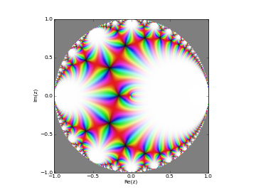
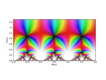
Evaluates the Klein j-invariant, which is a modular function defined for \(\tau\) in the upper half-plane as

\[J(\tau) = \frac{g_2^3(\tau)}{g_2^3(\tau) - 27 g_3^2(\tau)}\]

where \(g_2\) and \(g_3\) are the modular invariants of the Weierstrass elliptic function,

\[ \begin{align}\begin{aligned}g_2(\tau) = 60 \sum_{(m,n) \in \mathbb{Z}^2 \setminus (0,0)} (m \tau+n)^{-4}\\g_3(\tau) = 140 \sum_{(m,n) \in \mathbb{Z}^2 \setminus (0,0)} (m \tau+n)^{-6}.\end{aligned}\end{align} \]

An alternative, common notation is that of the j-function \(j(\tau) = 1728 J(\tau)\).

The half-period ratio may be supplied directly as tau, or through any of the argument forms accepted by qfrom(). The invariant can also be computed directly from Weierstrass invariants by providing both g2 and g3.

Plots

# Klein J-function as function of the number-theoretic nome
fp.cplot(lambda q: fp.kleinj(qbar=q), [-1,1], [-1,1], points=50000)

# Klein J-function as function of the half-period ratio
fp.cplot(lambda t: fp.kleinj(tau=t), [-1,2], [0,1.5], points=50000)

Examples

Verifying the functional equation \(J(\tau) = J(\tau+1) = J(-\tau^{-1})\):

>>> from mpmath import (mp, j, kleinj, taylor, sqrt, extraprec,
...                     chop, identify, cbrt)
>>> mp.dps = 25
>>> mp.pretty = True
>>> tau = 0.625+0.75*j
>>> tau = 0.625+0.75*j
>>> kleinj(tau)
(-0.1507492166511182267125242 + 0.07595948379084571927228948j)
>>> kleinj(tau+1)
(-0.1507492166511182267125242 + 0.07595948379084571927228948j)
>>> kleinj(-1/tau)
(-0.1507492166511182267125242 + 0.07595948379084571927228946j)

The j-function has a famous Laurent series expansion in terms of the nome \(\bar{q}\), \(j(\tau) = \bar{q}^{-1} + 744 + 196884\bar{q} + \ldots\):

>>> taylor(lambda q: 1728*q*kleinj(qbar=q), 0, 5, singular=True)
[1.0, 744.0, 196884.0, 21493760.0, 864299970.0, 20245856256.0]

The j-function admits exact evaluation at special algebraic points related to the Heegner numbers 1, 2, 3, 7, 11, 19, 43, 67, 163:

>>> @extraprec(10)
... def h(n):
...     v = (1+sqrt(n)*j)
...     if n > 2:
...         v *= 0.5
...     return v
...
>>> mp.dps = 25
>>> for n in [1,2,3,7,11,19,43,67,163]:
...     n, chop(1728*kleinj(h(n)))
...
(1, 1728.0)
(2, 8000.0)
(3, 0.0)
(7, -3375.0)
(11, -32768.0)
(19, -884736.0)
(43, -884736000.0)
(67, -147197952000.0)
(163, -262537412640768000.0)

Also at other special points, the j-function assumes explicit algebraic values, e.g.:

>>> chop(1728*kleinj(j*sqrt(5)))
1264538.909475140509320227
>>> identify(cbrt(_))      # note: not simplified
'((100+sqrt(13520))/2)'
>>> (50+26*sqrt(5))**3
1264538.909475140509320227

mpmath.kleinjinv(J)

Evaluates a branch of the inverse Klein j-invariant.

Given a value \(J\), returns a half-period ratio \(\tau\) in the upper half-plane such that kleinj(tau) equals \(J\), up to numerical error. Since kleinj is invariant under modular transformations, the inverse is multivalued; this function returns one representative. The branch is determined by principal square/cube roots in the formula below; the returned value is one modularly equivalent preimage and is not canonicalized to a fundamental domain.

The implementation uses the classical inverse construction via the modular lambda function, described as Method 1 in the Wikipedia article at https://en.wikipedia.org/wiki/J-invariant#Inverse_functions.

It first converts from the normalized invariant \(J\) to \(j = 1728 J\), then solves

\[j = 256 (1 - x)^3 / x^2, \quad x = \lambda (1 - \lambda),\]

for \(lambda\). The half-period ratio is then obtained from

\[\tau = i K(1 - \lambda) / K(\lambda),\]

where \(K\) is the complete elliptic integral. Using

\[K(m) = \pi / (2 \operatorname{AGM}(1, \sqrt{1 - m})),\]

this is evaluated by the arithmetic-geometric mean formula

\[\tau = i \operatorname{AGM}(1, \sqrt{1 - \lambda}) / \operatorname{AGM}(1, \sqrt{\lambda}).\]

Different root choices give different modularly equivalent branches.

Examples

>>> from mpmath import mp, kleinj, kleinjinv, chop
>>> mp.dps = 25
>>> mp.pretty = True
>>> tau = 0.625+0.75j
>>> chop(kleinj(kleinjinv(kleinj(tau))) - kleinj(tau))
0.0
>>> kleinjinv(1)
(0.0 + 1.0j)